Visualize and understand GPU memory in PyTorch

You must be familiar with this message 🤬:

RuntimeError: CUDA out of memory. Tried to allocate 20.00 MiB (GPU 0; 7.93 GiB total capacity; 6.00 GiB already allocated; 14.88 MiB free; 6.00 GiB reserved in total by PyTorch)

While it's easy to see that GPU memory is full, understanding why and how to fix it can be more challenging. In this tutorial, we'll go step by step on how to visualize and understand GPU memory usage in PyTorch during training. We’ll also see how to estimate memory requirements and optimize GPU memory usage.

🔎 The PyTorch visualizer

PyTorch provides a handy tool for visualizing GPU memory usage:

import torch
from torch import nn

# Start recording memory snapshot history
torch.cuda.memory._record_memory_history(max_entries=100000)

model = nn.Linear(10_000, 50_000, device ="cuda")
for _ in range(3):
    inputs = torch.randn(5_000, 10_000, device="cuda")
    outputs = model(inputs)

# Dump memory snapshot history to a file and stop recording
torch.cuda.memory._dump_snapshot("profile.pkl")
torch.cuda.memory._record_memory_history(enabled=None)

Running this code generates a profile.pkl file that contains a history of GPU memory usage during execution. You can visualize this history at: https://pytorch.org/memory_viz.

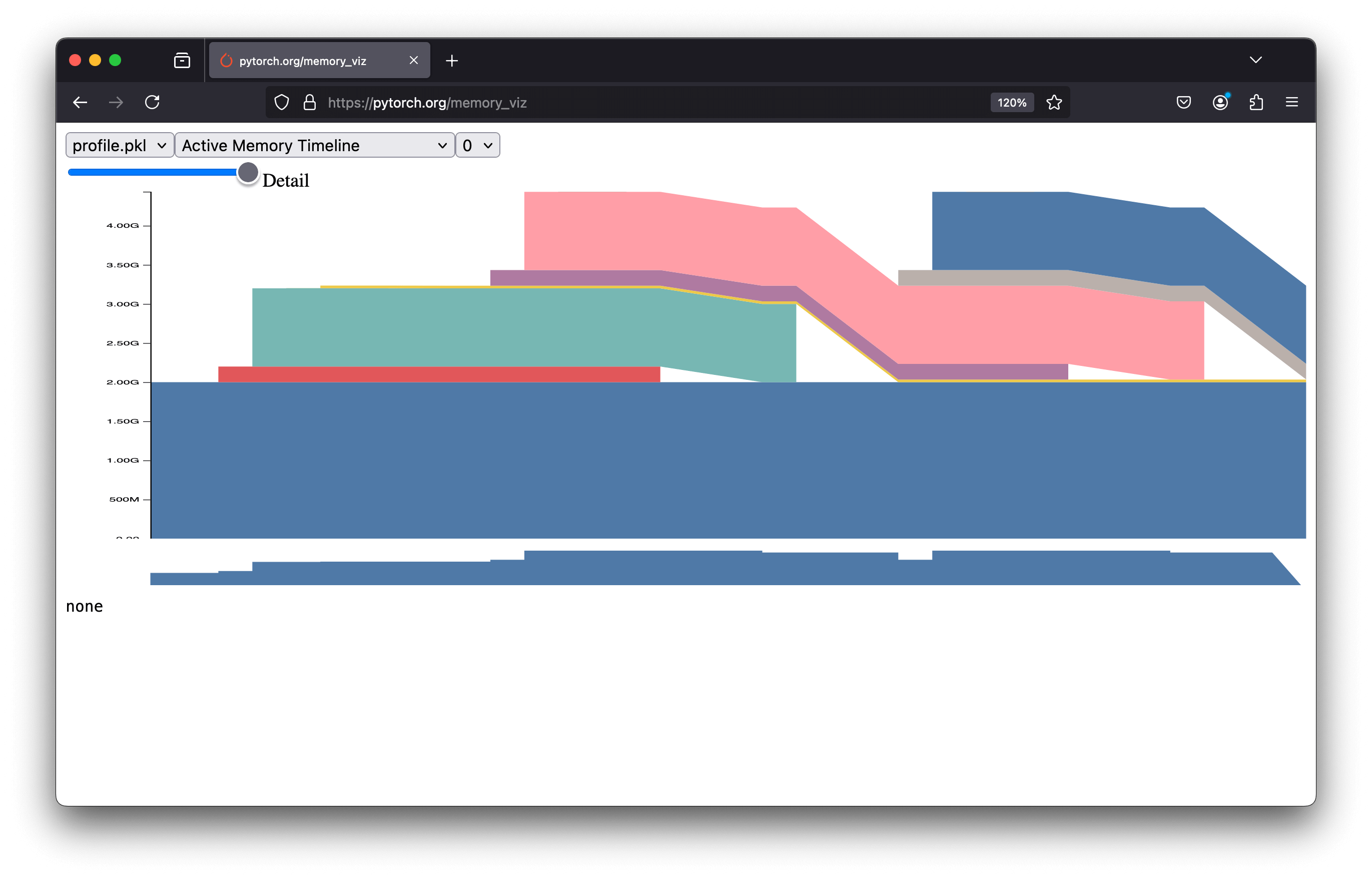
By dragging and dropping your profile.pkl file, you will see a graph like this:

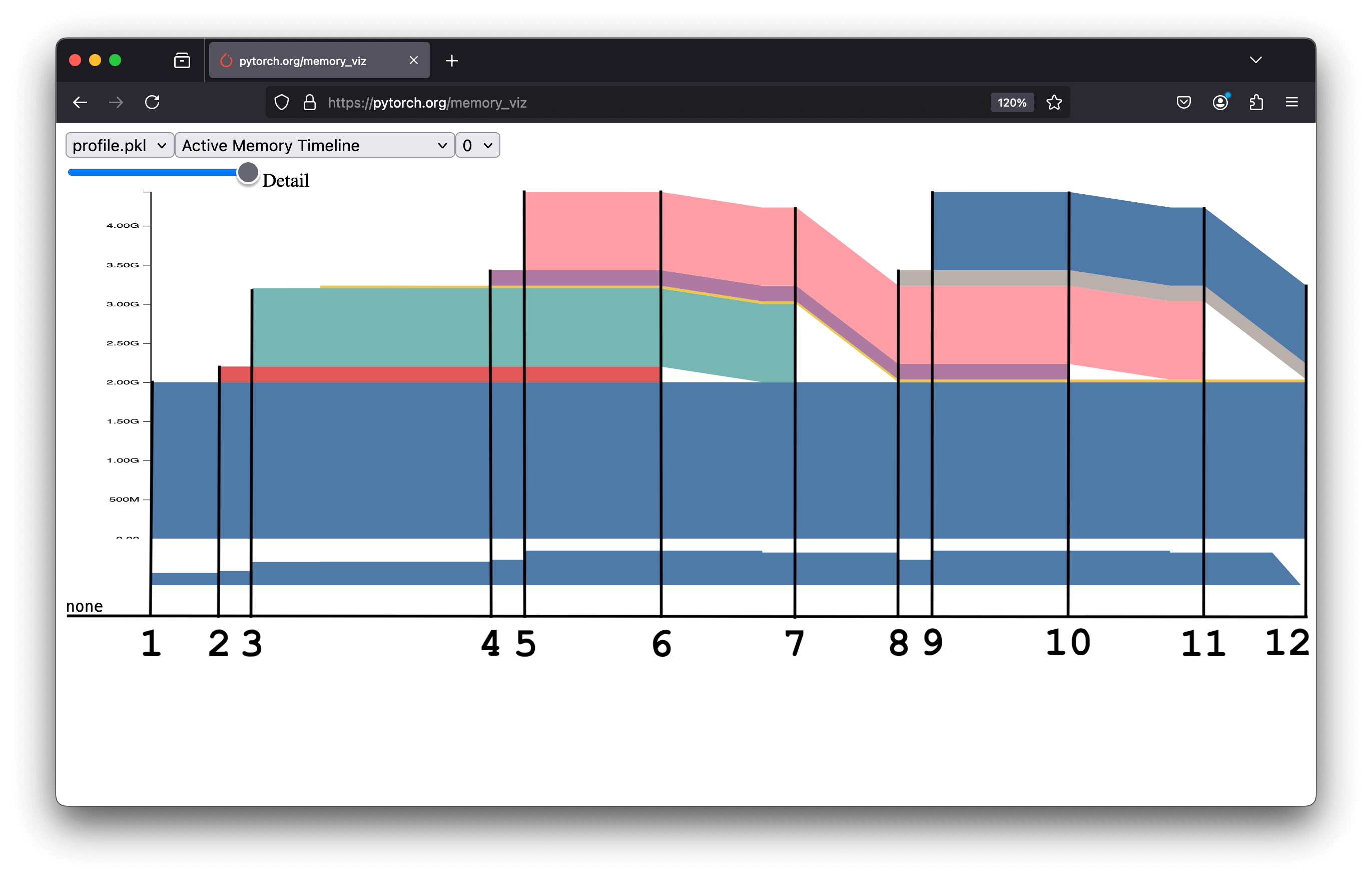
Let's break down this graph into key parts:

1. Model Creation: Memory increases by 2 GB, corresponding to the model's size:

   $10{,}000 \times 50{,}000 \text{ weights} + 50{,}000 \text{ biases in } \texttt{float32 }\text{(4 bytes)} \implies (5 \times 10^8) \times 4 \, \text{bytes} = 2 \, \text{GB}.$

   This memory (in blue) persists throughout execution.

2. Input Tensor Creation (1st Loop): Memory increases by 200 MB matching the input tensor size:

   $5{,}000 \times 10{,}000 \text{ elements in } \texttt{float32 }\text{(4 bytes)} \implies (5 \times 10^7) \times 4 \, \text{bytes} = 0.2 \, \text{GB}.$

3. Forward Pass (1st Loop): Memory increases by 1 GB for the output tensor:

   $5{,}000 \times 50{,}000 \text{ elements in } \texttt{float32 }\text{(4 bytes)} \implies (25 \times 10^7) \times 4 \, \text{bytes} = 1 \, \text{GB}.$

4. Input Tensor Creation (2nd Loop): Memory increases by 200 MB for a new input tensor. At this point, you might expect the input tensor from step 2 to be freed. Still, it isn't: the model retains its activation, so even if the tensor is no longer assigned to the variable inputs, it remains referenced by the model's forward pass computation. The model retains its activations because these tensors are required for the backpropagation process in neural networks. Try with torch.no_grad() to see the difference.

5. Forward Pass (2nd Loop): Memory increases by 1 GB for the new output tensor, calculated as in step 3.

6. Release 1st Loop Activation: After the second loop’s forward pass, the input tensor from the first loop (step 2) can be freed. The model's activations, which hold the first input tensor, are overwritten by the second loop's input. Once the second loop completes, the first tensor is no longer referenced and its memory can be released

7. Update output: The output tensor from step 3 is reassigned to the variable output. The previous tensor is no longer referenced and is deleted, freeing its memory.

8. Input Tensor Creation (3rd Loop): Same as step 4.

9. Forward Pass (3rd Loop): Same as step 5.

10. Release 2nd Loop Activation: The input tensor from step 4 is freed.

11. Update output Again: The output tensor from step 5 is reassigned to the variable output, freeing the previous tensor.

12. End of Code Execution: All memory is released.

📊 Visualizing Memory During Training

The previous example was simplified. In real scenarios, we often train complex models rather than a single linear layer. Additionally, the earlier example did not include the training process. Here, we will examine how GPU memory behaves during a complete training loop for a real large language model (LLM).

import torch
from transformers import AutoModelForCausalLM

# Start recording memory snapshot history
torch.cuda.memory._record_memory_history(max_entries=100000)

model = AutoModelForCausalLM.from_pretrained("Qwen/Qwen2.5-1.5B").to("cuda")
optimizer = torch.optim.AdamW(model.parameters(), lr=1e-3)

for _ in range(3):
    inputs = torch.randint(0, 100, (16, 256), device="cuda")  # Dummy input
    loss = torch.mean(model(inputs).logits)  # Dummy loss
    loss.backward()
    optimizer.step()
    optimizer.zero_grad()

# Dump memory snapshot history to a file and stop recording
torch.cuda.memory._dump_snapshot("profile.pkl")
torch.cuda.memory._record_memory_history(enabled=None)

💡 Tip: When profiling, limit the number of steps. Every GPU memory event is recorded, and the file can become very large. For example, the above code generates an 8 MB file.

Here’s the memory profile for this example:

This graph is more complex than the previous example, but we can still break it down step by step. Notice the three spikes, each corresponding to an iteration of the training loop. Let’s simplify the graph to make it easier to interpret:

1. Model Initialization (model = AutoModelForCausalLM.from_pretrained("Qwen/Qwen2.5-1.5B").to("cuda")):
   The first step involves loading the model onto the GPU. The model parameters (in blue) occupy memory and remain there until the training ends.

2. Forward Pass (model(inputs)):
   During the forward pass, the activations (intermediate outputs of each layer) are computed and stored in memory for backpropagation. These activations, represented in orange, grow layer by layer until the final layer. The loss is calculated at the peak of the orange zone.

3. Backward Pass (loss.backward()):
   The gradients (in yellow) are computed and stored during this phase. Simultaneously, the activations are discarded as they are no longer needed, causing the orange zone to shrink. The yellow zone represents memory usage for gradient calculations.

4. Optimizer Step (optimizer.step()):
   Gradients are used to update the model’s parameters. Initially, the optimizer itself is initialized (green zone). This initialization is only done once. After that, the optimizer uses the gradients to update the model’s parameters. To update the parameters, the optimizer temporarily stores intermediate values (red zone). After the update, both the gradients (yellow) and the intermediate optimizer values (red) are discarded, freeing memory.

At this point, one training iteration is complete. The process repeats for the remaining iterations, producing the three memory spikes visible in the graph.

Training profiles like this typically follow a consistent pattern, which makes them useful for estimating GPU memory requirements for a given model and training loop.

📐 Estimating Memory Requirements

From the above section, estimating GPU memory requirements seems simple. The total memory needed should correspond to the highest peak in the memory profile, which occurs during the forward pass. In that case, the memory requirement is (blue + greeen + orange): $\text{Model Parameters} + \text{Optimizer State} + \text{Activations}$

Is it that simple? Actually, there is a trap. The profile can look different depending on the training setup. For example, reducing the batch size from 16 to 2 changes the picture:

- inputs = torch.randint(0, 100, (16, 256), device="cuda")  # Dummy input
+ inputs = torch.randint(0, 100, (2, 256), device="cuda")  # Dummy input

Now, the highest peaks occur during the optimizer step rather than the forward pass. In this case, the memory requirement becomes (blue + green + yellow + red): $\text{Model Parameters} + \text{Optimizer State} + \text{Gradients} + \text{Optimizer Intermediates}$

To generalize the memory estimation, we need to account for all possible peaks, regardless of whether they occur during the forward pass or optimizer step. $\text{Model Parameters} + \text{Optimizer State} + \max(\text{Gradients} + {\text{Optimizer Intermediates}, \text{Activations}})$

Now that we have the equation, let's see how to estimate each component.

Model parameters

The model parameters are the easiest to estimate. $\text{Model Memory} = N \times P$

Where:

• $N$ is the number of parameters.
• $P$ is the precision (in bytes, e.g., 4 for float32).

For example, a model with 1.5 billion parameters and a precision of 4 bytes requires:

In the above example, the model size is: $\text{Model Memory} = 1.5 \times 10^9 \times 4 \, \text{bytes} = 6 \, \text{GB}$

Optimizer State

The memory required for the optimizer state depends on the optimizer type and the model parameters. For instance, the AdamW optimizer stores two moments (first and second) per parameter. This makes the optimizer state size: $\text{Optimizer State Size} = 2 \times N \times P$

Activations

The memory required for activations is harder to estimate because it includes all the intermediate values computed during the forward pass. To calculate activation memory, we can use a forward hook to measure the size of outputs:

import torch
from transformers import AutoModelForCausalLM

model = AutoModelForCausalLM.from_pretrained("Qwen/Qwen2.5-1.5B").to("cuda")

activation_sizes = []

def forward_hook(module, input, output):
    """
    Hook to calculate activation size for each module.
    """
    if isinstance(output, torch.Tensor):
        activation_sizes.append(output.numel() * output.element_size())
    elif isinstance(output, (tuple, list)):
        for tensor in output:
            if isinstance(tensor, torch.Tensor):
                activation_sizes.append(tensor.numel() * tensor.element_size())

# Register hooks for each submodule
hooks = []
for submodule in model.modules():
    hooks.append(submodule.register_forward_hook(forward_hook))

# Perform a forward pass with a dummy input
dummy_input = torch.zeros((1, 1), dtype=torch.int64, device="cuda")
model.eval()  # No gradients needed for memory measurement
with torch.no_grad():
    model(dummy_input)

# Clean up hooks
for hook in hooks:
    hook.remove()

print(sum(activation_sizes))  # Output: 5065216

For the Qwen2.5-1.5B model, this gives 5,065,216 activations per input token. To estimate the total activation memory for an input tensor, use: $\text{Activation Memory} = A \times B \times L \times P$

Where:

• $A$ is the number of activations per token.
• $B$ is the batch size.
• $L$ is the sequence length.

However, using this method directly isn't always practical. Ideally, we would like a heuristic to estimate activation memory without running the model. Plus, we can intuitively see that larger models have more activations. This leads to the question: Is there a connection between the number of model parameters and the number of activations?

Not directly, as the number of activations per token depends on the model architecture. However, LLMs tend to have similar structures. By analyzing different models, we observe a rough linear relationship between the number of parameters and the number of activations:

This linear relationship allows us to estimate activations using the heuristic: $A = 4.6894 \times 10^{4} \times N + 1.8494 \times 10^{6}$

Though this is an approximation, it provides a practical way to estimate activation memory without needing to perform complex calculations for each model.

Gradients

Gradients are easier to estimate. The memory required for gradients is the same as the model parameters: $\text{Gradients Memory} = N \times P$

Optimizer Intermediates

When updating the model parameters, the optimizer stores intermediate values. The memory required for these values is the same as the model parameters: $\text{Optimizer Intermediates Memory} = N \times P$

Total Memory

To summarize, the total memory required to train a model is: $\text{Total Memory} = \text{Model Memory} + \text{Optimizer State} + \max(\text{Gradients}, \text{Optimizer Intermediates}, \text{Activations})$

with the following components:

• Model Memory: $N \times P$
• Optimizer State: $2 \times N \times P$
• Gradients: $N \times P$
• Optimizer Intermediates: $N \times P$
• Activations: $A \times B \times L \times P$, estimated using the heuristic $A = 4.6894 \times 10^{4} \times N + 1.8494 \times 10^{6}$

To make this calculation easier, I created a small tool for you:

🚀 Next steps

Your initial motivation to understand memory usage was probably driven by the fact that one day, you ran out of memory. Did this blog give you a direct solution to fix that? Probably not. However, now that you have a better understanding of how memory usage works and how to profile it, you're better equipped to find ways to reduce it.

For a specific list of tips on optimizing memory usage in TRL, you can check the Reducing Memory Usage section of the documentation. These tips, though, are not limited to TRL and can be applied to any PyTorch-based training process.

🤝 Acknowledgements

Thanks to Kashif Rasul for his valuable feedback and suggestions on this blog post.